机器学习数学基础-回归

回归

作为一次函数实现

import numpy as np
import matplotlib.pyplot as plt

读入训练数据

train = np.loadtxt('click.csv', delimiter=',', skiprows=1)
train_x = train[:,0]
train_y = train[:,1]

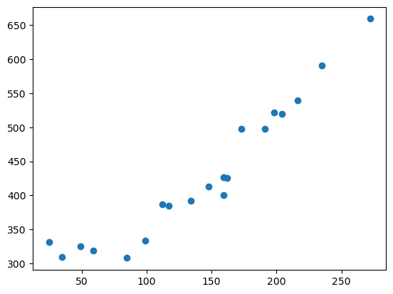
画图展示

plt.plot(train_x, train_y, 'o')

[<matplotlib.lines.Line2D at 0x7fc95f6b1410>]

初始化函数

$f_\theta (x)=\theta_0 + \theta_1 x$

$E(\theta) = \frac{1}{2}\sum\limits_{i=1}^{n} (y^{(i)}-f_\theta(x^{(i)}))^2$

编写 $f_\theta(x)$

theta0 = np.random.rand()
theta1 = np.random.rand()
def f(x):
    return theta0 + theta1 * x

编写 $E(\theta)$

def E(x, y):
    return 0.5 * np.sum((y - f(x)) ** 2)

z-score规范化 (标准化)

把训练数据变成平均值为0、方差为 1 的数据。这项操作有利于加快参数的收敛。

$z^{(i)} = \frac{x^{(i)}-\mu}{\sigma}$

其中 $\mu$ 是训练数据的平均值，$\sigma$ 是标准差(方差的算数平方根)。

mu = train_x.mean() # numpy中mean()函数用于求取平均值
sigma = train_x.std() # numpy中std()函数用于求解标准差

def standarize(x):
    return (x - mu) / sigma

train_z = standarize(train_x)

展示标准化之后的数据：

plt.plot(train_z, train_y, 'o')
plt.show()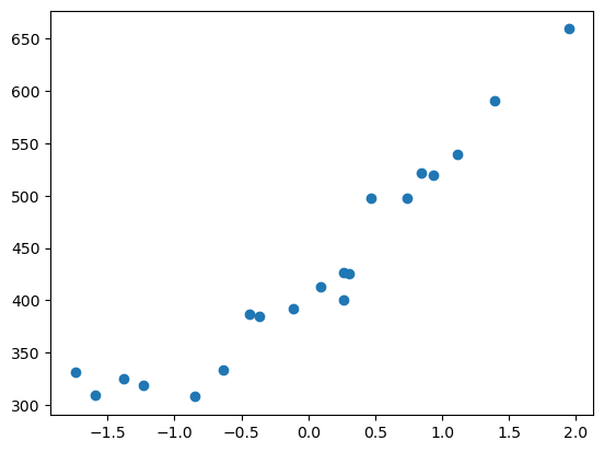

参数更新

$\theta_0 := \theta_0 - \eta\sum\limits_{i=1}^{n}(f_\theta(x^{(i)}) - y^{(i)})$

$\theta_1 := \theta_1 - \eta\sum\limits_{i=1}^{n}(f_\theta(x^{(i)}) - y^{(i)})x^{(i)}$

# 曾经在此出错，jupyter要重复演示这段代码应该将随机参数写在此处
theta0 = np.random.rand()
theta1 = np.random.rand()

ETA = 1e-3 # 学习率
diff = 1 # 误差差值
count = 0 # 更新次数
error = E(train_z, train_y)
while diff >= 1e-2:
    # 注意：更新参数时要两个同时一起更新，否则更新第二个参数时会使用已更新的theta0
    tmp0 = theta0 - ETA * np.sum((f(train_z) - train_y))
    tmp1 = theta1 - ETA * np.sum((f(train_z) - train_y) * train_z)
    theta0 = tmp0
    theta1 = tmp1
    # 计算与上一次误差的差值(即误差减少量)
    current_error = E(train_z, train_y)
    diff =  error - current_error # 曾经在此出错，写反会导致误差是负数
    error = current_error

    count += 1
    log = ' 第 {} 次 : theta0 = {:.3f}, theta1 = {:.3f}, 差值 = {:.4f}'
    print(log.format(count, theta0, theta1, diff))
    

 第 1 次 : theta0 = 8.958, theta1 = 2.110, 差值 = 76243.2366
 第 2 次 : theta0 = 17.362, theta1 = 3.938, 差值 = 73224.0044
 ...
 第 393 次 : theta0 = 428.997, theta1 = 93.446, 差值 = 0.0101
 第 394 次 : theta0 = 429.000, theta1 = 93.446, 差值 = 0.0097

x = np.linspace(-3, 3, 100) # 生成[-3,3]间均匀的100个数, 用于函数图像
plt.plot(train_z, train_y, 'o')
plt.plot(x, f(x))
plt.show()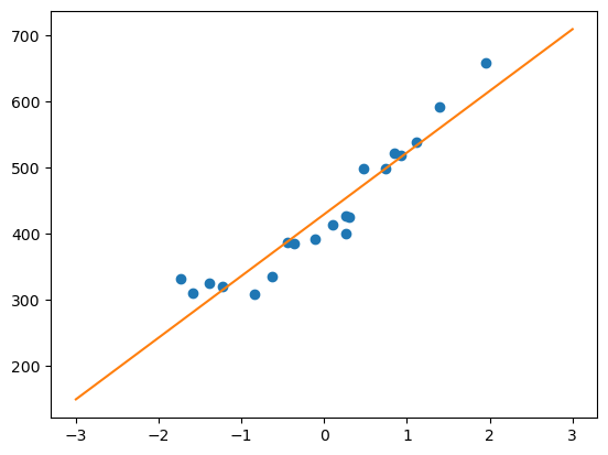

多项式回归

一般化 $f_\theta(x)$

$f_\theta(x)=\theta_0+\theta_1x+\theta_2x^2$

将参数和训练数据都作为向量来处理，可以使计算变得更简单。

由于训练数据有很多，所以将每一行数据都视作一个训练数据，以矩阵的形式来处理。

$\mathbf{X}=\begin{bmatrix}x^{(1)^T}\\x^{(2)^T}\\x^{(3)^T}\\\dots\\x^{(n)^T}\end{bmatrix}=\begin{bmatrix}1&x^{(1)}&x^{(1)^2}\\1&x^{(2)}&x^{(2)^2}\\1&x^{(3)}&x^{(3)^2} \\\dots\\1&x^{(n)}&x^{(n)^2}\end{bmatrix}$

于是我们只用求出矩阵与参数向量 $\mathbf{\theta}$ 的乘积。

$f_\theta(x)=\mathbf{X}\mathbf{\theta}$

theta = np.random.rand(3) # 直接生成出3个随机数的向量

# 将数据存放在矩阵中
def to_matrix(x):
    '''
    np.ones(x.shape[0]) 创建一个长度为 x 的数组, 元素全部为1, 表示常数项。
    np.vstack(...) 将上述三个数组垂直堆叠, 完成这一步后矩阵变为：
        [[1,1,...,1],
         [x1,x2,...,xn],
         [x1^2,x2^2,...,xn^2]]
    后缀 .T 表示转置
    '''
    return np.vstack([np.ones(x.shape[0]), x, x**2]).T

def f(x):
    return np.dot(x, theta) # 用于执行矩阵乘法（矩阵点积）的函数

一般化参数更新

已推出:

$\theta_j := \theta_j - \eta\sum\limits_{i=1}^{n}(f_\theta(x^{(i)}) - y^{(i)})x_j^{(i)}$

把表达式中 $f_\theta(x^{(i)}) - y^{(i)}$ 和 $x_j^{(i)}$ 的部分分别当作向量来处理。

通过向量相乘可直接表示:

$\theta_j := \theta_j - \mathbf{f}^T\mathbf{X}$

为方便理解向量积有下例:

$\mathbf{a}=\begin{bmatrix}2\\5\\2\end{bmatrix},\mathbf{b}=\begin{bmatrix}1\\2\\3\end{bmatrix}$ 则 $\mathbf{a}^Tb=\begin{bmatrix}2 5 2\end{bmatrix}\begin{bmatrix}1\\2\\3\end{bmatrix}=\begin{bmatrix}2×1+5×2+2×3\end{bmatrix}=\begin{bmatrix}18\end{bmatrix}$

diff = 1
X = to_matrix(train_z)
error = E(X, train_y)
while diff >= 1e-2:
    theta = theta - ETA * np.dot(f(X) - train_y, X)
    current_error = E(X, train_y)
    diff = error - current_error
    error = current_error

展示

x = np.linspace(-3, 3, 100) # 生成[-3,3]间均匀的100个数, 用于函数图像
plt.plot(train_z, train_y, 'o')
plt.plot(x, f(to_matrix(x)))
plt.show()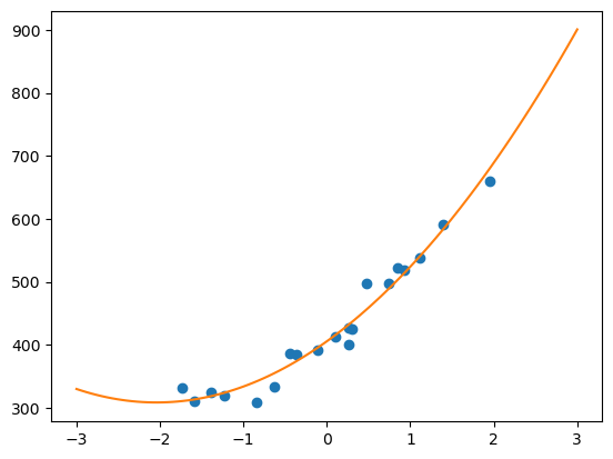

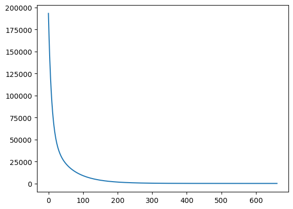
误差变化可视化

均方误差 $MSE = \frac{1}{n}\sum\limits^n_{i=1}(y^{(i)} - f_\theta(\mathbf{x}^{(i)}))^2$

def MSE(x, y):
    return (1 / x.shape[0]) * np.sum((y - f(x)) ** 2)

theta = np.random.rand(3)
errors = []
diff = 1

errors.append(MSE(X, train_y))
while diff > 1e-2:
    theta = theta - ETA * np.dot(f(X) - train_y, X)
    errors.append(MSE(X, train_y))
    diff = errors[-2]- errors[-1]

# 绘图
x = np.arange(len(errors))

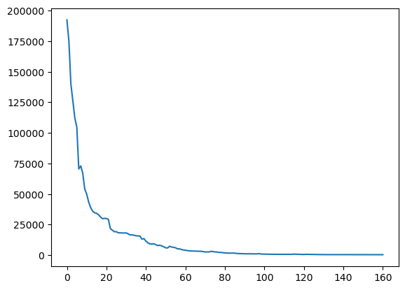
plt.plot(x, errors)

[<matplotlib.lines.Line2D at 0x7fc95f411c50>]

随机梯度下降法

$\theta_j := \theta_j - \eta\sum\limits_{i=1}^{n}(f_\theta(x^{(k)}) - y^{(i)})x_j^{(k)}$

p = np.random.permutation(X.shape[0])
print(p)

[10 16  2 18  0  6  3 11  7  5  4  9  1 15 13 12 17  8 14 19]

theta = np.random.rand(3)
errors = []  # 均方误差
diff = 1
errors.append(MSE(X, train_y))
ETA = 0.05

while diff > 1e-3:
    # 随机取出数据, 取长度时就是打乱数据
    p = np.random.permutation(X.shape[0])
    for x, y in zip(X[p,:], train_y[p]):
        # 此处不应该用点积，因为已经进入了循环，相当于小部分取样的点积
        theta = theta - ETA * (f(x) - y) * x
        errors.append(MSE(X, train_y))
        diff = errors[-2] - errors[-1]

# 绘图确认
x = np.linspace(-3, 3, 100)  # 生成[-3,3]间均匀的100个数, 用于函数图像
plt.plot(train_z, train_y, "o")
plt.plot(x, f(to_matrix(x)))
plt.show()

# 绘图
x = np.arange(len(errors))

plt.plot(x, errors)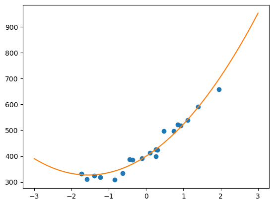

[<matplotlib.lines.Line2D at 0x7fc95e98c090>]